Normal Forms Methods

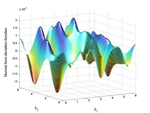
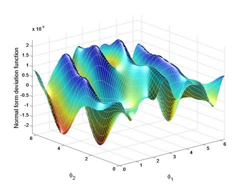
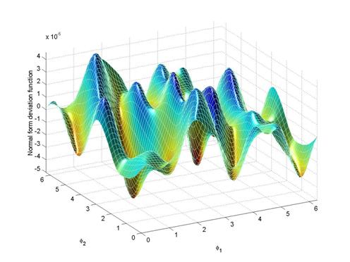
The polynomials that generate the normal form pictures can be found below in two versions, one consisting of polynomials of order five, the other of polynomials of order ten.

The normal form defect function has the form


D = I (A P B ) - I


Where I is a single polynomial in six variables, and A, P, and B each are six polynomials in six variables that are composed. The total of 19(=1+6+6+6) polynomials are listed consecutively, in the order I, A1 … A6,  P1 … P6, B1 … B6.


Fifth Order Version 

Tenth Order Version

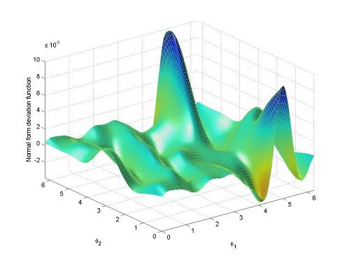
     Normal form methods are a very useful tool for the study of the local dynamics of nonlinear systems around fixed points. In particular, the so-called normal form defect function, which describes the evolution of an approximate invariant of the motion, provides significant insight into the dynamics. If the function can be proven to be strictly less than zero over a given domain, it constitutes a Lyapunov function, and the system is guaranteed to be stable. For Hamiltonian systems or other volume-preserving systems, the normal form function is never strictly zero; but the magnitude of its usually very small positive bound allow to put rather extended bounds on stability times of the dynamics.

     The pictures show two dimensional projections of the normal form defect function for a six dimensional Hamiltonian system. The approximate invariant consists of a composition of three polynomials in six variables of order five, which can be found here. The two variables are the angles f
1 and f2  varying from 0 to 2 pi of a polar coordinate representation of the positions and momenta (q,p).

     The pictures show the resulting information for the following four cases:

r
1=0.1, r2 = 0.1, r3 = 0.1,   f3 = pi  (viewpoint 1)
r
1=0.1, r2 = 0.1, r3 = 0.1,   f3 = pi  (viewpoint 2)
r
1=0.1, r2 = 0.1, r3 = 0.15, f3 = pi
r
1=0.1, r2 = 0.1, r3 = 0.1,   f3 = pi

     Note the scale of the function values, which is in the range of 10
-5, attesting to the quality of the pseudo invariant.

     From a computational point of view, the bounding of the normal form defect function represents a formidable challenge; there are large numbers of local extrema, and the function itself consists of a very large number of terms. Within the framework of theorem proving, bounds have to be established rigorously, for which we utilize the Taylor model methods developed at MSU. These tools lead to a savings in computation time of many orders of magnitude compared to other validated methods, and for higher-dimensional normal form problems represent the only known tools that allow their rigorous bounding.